How to Highlight the Lowest Value in Excel

Highlighting the lowest value in an Excel spreadsheet is a fundamental skill that can significantly enhance data analysis and visualization. This simple yet powerful technique allows you to quickly identify key data points, trends, and outliers within your datasets. Whether you’re tracking sales figures, analyzing student grades, or managing inventory, knowing how to highlight the lowest value in Excel can save you time and improve your overall efficiency.

Pinpointing the Minimum: Various Methods to Highlight the Lowest Value

Excel offers several flexible methods to highlight the lowest value, each with its own advantages. Choosing the right method depends on your specific needs and the complexity of your data.

• Conditional Formatting: This is arguably the most versatile and commonly used method. Conditional formatting allows you to apply formatting rules based on specific criteria, such as highlighting the lowest value in a range. You can choose from a variety of formatting options, including changing the cell color, font color, or adding icons.

• Using the MIN Function: The MIN function allows you to identify the lowest numerical value within a specific range. While this function doesn’t directly highlight the cell, you can combine it with conditional formatting to achieve the desired result. This is particularly useful for dynamic data sets where the lowest value might change frequently.

• Manual Formatting: For smaller datasets, manually formatting the cell containing the lowest value might be the quickest option. Simply locate the lowest value and apply the desired formatting. However, this method is less efficient for larger datasets and is prone to human error.

Conditional Formatting: A Step-by-Step Guide to Highlight the Lowest Value

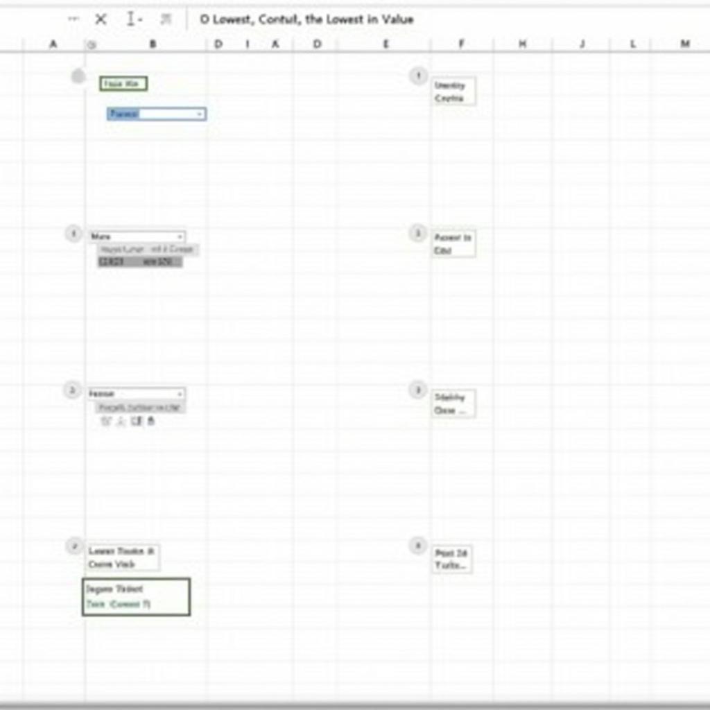
Let’s delve deeper into the most common method: conditional formatting. Here’s a step-by-step guide to highlight the lowest value in Excel using conditional formatting:

1. Select the Range: Select the cells containing the data you want to analyze.

2. Open Conditional Formatting: Go to the “Home” tab and click on “Conditional Formatting” in the “Styles” group.

3. Choose a Rule: Select “Highlight Cells Rules” and then choose “More Rules…”.

4. Select Format Style: In the “New Formatting Rule” dialog box, select “Format only top or bottom ranked values”.

5. Specify Bottom Ranked Value: Choose “Bottom” from the drop-down menu and enter “1” in the value box to highlight only the lowest value.

6. Customize Formatting: Click the “Format…” button to choose the desired formatting style (e.g., fill color, font color).

7. Click OK: Click “OK” to apply the formatting rule.

Using Conditional Formatting to Highlight the Lowest Value

Beyond the Basics: Advanced Techniques for Highlighting the Lowest Value

For more complex scenarios, you can use more advanced techniques, such as:

• Highlighting Multiple Lowest Values: If there are multiple cells with the same lowest value, you can adjust the conditional formatting rule to highlight all of them. Simply change the value in the “Format only top or bottom ranked values” dialog box to the number of lowest values you want to highlight.

• Highlighting the Lowest Value in Each Row or Column: To highlight the lowest value in each row or column, you can use a combination of the MIN function and conditional formatting.

• Using VBA for Complex Logic: For highly complex scenarios, you can utilize Visual Basic for Applications (VBA) to create custom macros that automate the highlighting process based on specific criteria. Similar to how you might highlight one row in pivot table with conditional formatting, VBA offers greater flexibility and control.

Advanced Techniques for Highlighting Lowest Value in Excel

Conclusion

Highlighting the lowest value in Excel is a simple yet effective technique for data analysis. Whether you use conditional formatting, the MIN function, or manual formatting, this skill can help you quickly identify key data points and improve your decision-making process.

FAQ

1. Can I highlight the lowest value with a specific color? Yes, you can customize the formatting to use any color you prefer.
2. What if my data contains text and numbers? Conditional formatting will only consider numerical values when determining the lowest value.
3. Can I highlight the lowest value in a non-contiguous range? Yes, you can select multiple non-adjacent ranges before applying conditional formatting.
4. Can I highlight the second lowest value? Yes, you can adjust the conditional formatting rule to highlight any ranked value.
5. Does this work on different versions of Excel? Yes, these methods are generally applicable across different Excel versions.
6. What if my data changes frequently? Conditional formatting will automatically update the highlighting based on the new data.
7. Can I highlight the lowest value across multiple worksheets? Yes, but it requires a more complex formula or VBA.

Khi cần hỗ trợ hãy liên hệ Số Điện Thoại: 0372999996, Email: [email protected] Hoặc đến địa chỉ: 236 Cầu Giấy, Hà Nội. Chúng tôi có đội ngũ chăm sóc khách hàng 24/7.